We all know about the concept of motion and how it helps us in developing scientific understanding. Rectilinear motion is the motion of a particle in a straight line. It is the simplest type of motion often studied in physics.
The frame of reference is an important concept when we want to study any kind of motion. It allows us to define the positions and velocities of objects relative to a particular observer or coordinate system.
In this article, we will look at the idea of rectilinear motion and methodologies used to find the equation of motion governing the motion of a moving object.
The Basics of Rectilinear Motion
Rectilinear motion occurs when an object moves in a straight line. For simplification, we can align a coordinate axis (e.g., the x-axis) along the object’s path. At any given moment, the moving object has a definite coordinate relative to the reference frame.
The object’s coordinate is a function of time, expressed as x = f(t), and the form of this function represents the equation of motion.
How we determine motion equations experimentally
To experimentally determine motion equations, we need to mark an object’s position on the coordinate axis at specific time intervals.
Consider a moving car as an example. We could place markers along the road and record the car’s position relative to the markers at equal time intervals. The table given below shows the results of our experiment. We will use this data to understand the motion of the car at different instants of time.
| Instant of time $t$ in seconds | 1 | 2 | 3 | 4 | 5 | 6 | 7 | 8 |
|---|---|---|---|---|---|---|---|---|
| Coordinate $x$ in meter | 1 | 1.25 | 1.50 | 1.75 | 2.00 | 2.25 | 2.50 | 2.75 |
It is important to note here that our experiment has not given us the reliable information about the position of the object at intermediate moments for example the moments between $1 s$ and $2 s$.
To overcome this problem we can consider using these recorded positions to find a function x = f(t) that best represents the car’s motion. It goes without saying that that matches the given data points, where t represents time and x represents the position of the object at that time.
Now from the data in the table, we can clearly see that
- When $t = 1s, x = 1m$
- When $t = 2s, x = 1.25m$
- When $t = 3s, x = 1.50m$ and so on
By looking at this data we can intuitively try to find the function $x=f(t)$ such that when we substitute values for $t=1,2, 3, 4…..$ in that function, we get exactly the same values of $x$ as measured during the experiment as the output of that function.
By looking at the data it can be seen that it is a linear function of $x$ such that it corresponds exactly to the provided data points.
$x=f(t)=1+0.25t$
If the object’s motion is consistent then this function can be used to calculate the x-coordinate (position) for any moment between the first and eighth second (the time interval of interest).
The Importance of Time Intervals and Volume of Information
The accuracy of motion equations relies heavily on the volume of information available. The more marks we have and the shorter the time intervals between successive marks, the more accurately we can determine the motion equations. When conducting experiments, it is crucial to collect sufficient data to ensure the motion equations are as close to the truth as possible.
Now considering the previous example of the moving car the motion equation derived from experimental data is only valid for the time interval during which the investigation was conducted. In other words, the motion equation accurately describes the car’s motion as long as the conditions (e.g., the car’s speed) remain consistent throughout the experiment.
Extrapolation refers to using the motion equation to predict the car’s position beyond the investigated time interval. This can be risky if the character of motion changes, as the motion equation may not accurately describe the car’s behavior outside the experimental time frame.
To ensure the motion equation’s validity for a longer time interval, supplementary investigations are necessary. These additional investigations aim to confirm that the character of motion remains unchanged, allowing for the accurate application of the motion equation beyond the initial experimental time frame.
Limitations of Motion Equations and the Need for Supplementary Investigations
The motion equations determined from experiments are only valid for the time interval during which the investigation was conducted. So it is important for us to maintain the consistent characteristics of motion throughout the experiment to ensure the validity of the motion equations derived from the experimental data.
If the character of motion changes (e.g., if the car’s speed changes), the motion equations may not accurately describe the motion beyond the investigated time interval. Extrapolating these equations is only permissible after supplementary investigations to establish that the character of motion remained unchanged.
Let’s consider the car example mentioned in the previous section. We assume that the character of motion (in this case, the speed of the car) does not change during the experiment to derive an accurate motion equation.
Suppose, after a specific point in time (let’s say after 10 seconds), the driver decides to accelerate or decelerate the car. This change in speed alters the character of the car’s motion, and the previously determined motion equation is no longer valid for the time after the 10th second.
In this situation, using the initial motion equation to predict the car’s position after the change in speed would result in inaccurate estimations. To determine a new motion equation that accurately describes the car’s motion after the change in speed, we would need to conduct another experiment or gather additional data under the new conditions.
Conclusion
Rectilinear motion is a fundamental concept in physics, and understanding it requires knowledge of motion equations and the frame of reference. By conducting experiments and collecting accurate data, we can determine motion equations that accurately describe an object’s motion.
As we continue to explore the complexities of motion, a strong foundation in these concepts will help us unlock new scientific and technological breakthroughs.


